O’Brien, R., & Ishwaran, H. (2019). A random forests quantile classifier for class imbalanced data. Pattern recognition, 90, 232-249.

In Short

불균형데이터 처리를 위해, quantile classifier을 사용한 Random Forest

1. Introduction

1-1. 불균형데이터의 정의

일반적으로 두 개의 클래스가 있는 상황에서, 한 클래스에 속한 원소가 나머지 클래스에 속한 원소에 비해 월등하게 많은 경우를 데이터가 불균형한 상황이라고 정의한다. (여기서는 $Y=1$이 Minoritiy, $Y=0$이 Majority라고 생각하자.)

5개의 근접원소들에 대해서 Majority 클래스에 속하는 원소가 0~1개인 원소를 Safe, 2~3개는 Borderline, 4~5개는 Rare라고 부른다.

1-2. IR (Imbalance Ratio)

$$IR = \frac{\text{# of Majority class}}{\text{# of Minority class}}$$

1-3. Marginally imbalanced

정의: $p(x) \ll \frac{1}{2} \text{ for all } x \in X \text{ where } p(x) = P(Y=1|X=x)$
포인트는 all x인 것 같다. 모든 데이터에 대해서 특정 클래스(소수 클래스)일 확률이 극단적으로 작을 경우 marginally imbalanced라고 한다.

1-4. Conditionally imbalanced

정의: $\text{there exists a set } A \subset X \text{ with nonzero probability, } P(X \in A) >0, \text{ such that } P(Y=1|X \in A) \approx 1 \text{ and } p(x) \ll \frac{1}{2} \text{ for } x \notin A$
특정 데이터셋에 대해서는 소수 클래스일 확률이 1에 가깝지만, 그외 대부분의 데이터셋에 대해서는 소수 클래스일 확률이 0에 가까운 경우를 conditionally imbalanced라고 하는 것 같다. 개인적으로 1-3의 marginallly imbalanced보다는 conditionally imbalanced가 조금 더 현실적인 데이터의 특성을 더 반영했다고 생각은 든다.

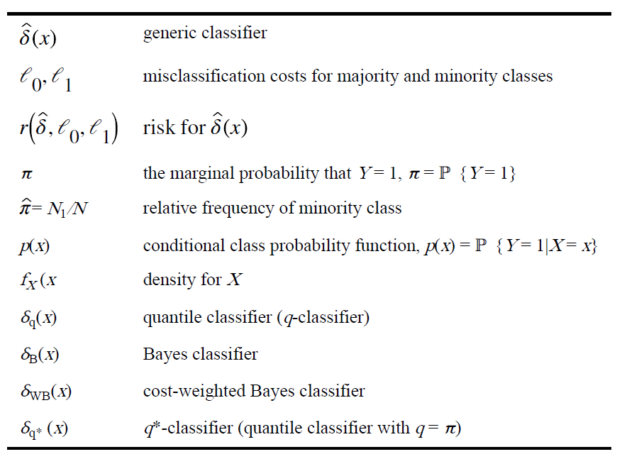
1-5. Notation 정리

아래는 본 논문의 Table 1이다.

2. Related Work

2-1. Data Level Methods

데이터 자체를 건드려서 해결하는 방식을 Data Level Method라고 칭한다. 본 논문에서 이야기하는 대표적인 예시로는 Balanced Random Forest(BRF)가 있다. 이는 다수 클래스에 속하는 것들을 적게 뽑는(undersampling) 방식이다. 이외에 SMOTE와 같은 oversampling 기법들도 있고, undersampling과 oversampling이 결합된 하이브리드 방식도 있다. 아래는 해당 논문에서 추가적으로 언급된 방법론들이다.

• One-sided Sampling: Tomek Links
• Neighborhood Balanced Bagging
• SMOTEBoost, RUSBoost, EUSBoost: combine boosting with sampling data at each boosting iteration

2-2. Algorithmic Level Methods

위처럼 데이터의 균형을 직접적으로 조절하는 방식이 있는가하면, 알고리즘적으로 분류 성능을 높이고자 하는 노력들도 있었다. 아래는 다양한 방법론들 예시이다.

• SHRINK
• Helling Distance Decision Trees(HDDT)
• Near-Bayesian Support Vector Machines(NBSVM)
• Class Switching according to NEarest Enemy Distance

2-3. Bayes Decision Rule

$$\delta_B(x) = I\big( p(x) \geq 1/2 \big)$$
참고로 여기서 $p(x) = P(Y=1 | X=x)$이다. 이는 IR이 커지면 문제가 된다. $p(x)$가 0에 가까우면 해당 classifier는 Majority 클래스로 예측하게 되는데, 일반적으로 다수의 원소가 속해있는 클래스로 예측하도록 $p(x)$가 0에 가깝게 되는 경우가 많기 때문이다. 그리고 이때 Bayes error는 아래와 같이 0에 가깝게 나오므로 마치 완벽한 분류기처럼 착각될 수 있다.
$$r(\delta_B) = E[\min\{p(X), 1-p(X)\}] = E[p(X)] \approx 0$$

2-4. Balanced Random Forests (BRF)

random forests with undersampling the majority class

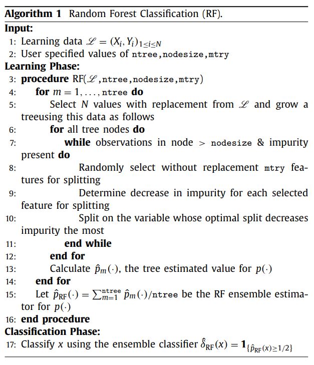
2-5. Algorithm Procedure of Random Forest Classification

3. Q*-Classifier

3-1. Quantile classifier

$$\delta_q(x) = I\big( p(x) \geq q \big), \ 0<q<1$$
quantile classifer가 무엇인지 이해하면, 해당 논문의 핵심 포인트인 q*-classifier을 이해할 수 있다.

해당 방법론은 크게 두 가지 장점이 있다. 첫번째는 TPR과 TNR을 최대화한다는 점이다. 두번째는 cost-weighted Bayes classifier과 같이 작동함으로써 weighted risk를 최소화해준다.

$$r(\hat{\delta}, \ell_0, \ell_1) = E\Big[\ell_{0}1_{(\hat{\delta}(X)=1, Y=0)} + \ell_{1}1_{(\hat{\delta}(X)=0, Y=1)}\Big]$$

여기서 $\ell_0$와 $\ell_1$은 각각 Majority 원소 또는 Minority 원소를 잘못 분류할 때의 cost이며, 모두 양수이다.

cost-weighted risk의 관점에서 보면, 최적의 classifier는 cost-weighted Bayes rule을 활용하는 것인데, 이는 아래와 같이 나타낼 수 있다.
$$\delta_{WB}(x) = 1_{\big(p(x) \geq \frac{\ell_0}{\ell_0 + \ell_1}\big)}$$

위에 대한 증명은 논문 Appendix1에 정리되어있으며, 추후 추가 서술하도록 하겠다.

3-2. TNR+TPR optimal

TNR(True Negative Rate)와 TPR(True Positive Rate)의 합을 최대화시켜주는 분류기를 TNR+TPR optimal이라고 부른다.
$$TPR = \frac{TP}{TP+FN}, \ TNR = \frac{TN}{TN+FP}$$
참고로 기본 Bayes Rule을 활용한 분류기는 TNR은 1에 가깝지만, TPR은 0에 가깝게 나온다는 한계가 있다.

3-3. q*-classifier

$$\delta_D(x) = 1_{\big(\Delta_D(x) \geq 1\big)} \text{, where } \Delta_D(x) = \frac{f_{X|Y}(x|1)}{f_{X|Y}(x|0)} = \frac{p(x)(1-\pi)}{(1-p(x))\pi} \qquad (4)$$

여기서 $\delta_{q*}(x) = I\big(p(x) \geq \pi \big) = \delta_D(x)$를 q*-classifier라고 부른다. 이는 알고리즘적으로 데이터 불균형 문제를 해결하고자 하는 방법에 속하며, Density-based approach라고 할 수 있다. 왜냐하면 data density를 활용하여 클래스를 분류하기 때문이다.

cf. Density-based approach
$$\delta_D(x) = 1_{\big(f_{X|Y}(x|1) \geq f_{X|Y}(x|0)\big)}$$
여기서 주목해야 할 점은 conditional density of the response ($p(x)$)가 아니라 conditional density of the features($f_{X|Y}$)를 활용했다는 점이다. 이로 인해 소수 클래스의 prevalance 효과를 제거할 수 있다. (개인생각: Bayesian의 용어로 해석한다면, 선행연구처럼 uniform prior가 아니라 likelihood를 기준으로 분류를 했다는 데에 의의가 있는 것 같다.)

Theorem2 중에서 TNR+TPR optimal에 대한 증명은 아래와 같다. 참고로, FPR = 1-TNR, FNR = 1-TPR이므로, TNR와 TPR을 최대화하는 것은 FPR과 FNR을 최소화하는 것과 같다.

\begin{align} FPR(\hat{\delta}) &+ FNR(\hat{\delta})\\ &= P\{\hat{\delta}(X)=1|Y=0\} + P\{\hat{\delta}(X)=0|Y=1\} \\ &= \frac{P\{\hat{\delta}(X)=1, Y=0\}}{P(Y=0)} + \frac{P\{\hat{\delta}(X)=0, Y=1\}}{P(Y=1)} \\ &= E\Big[\frac{1\{\hat{\delta}(X)=1, Y=0\}}{\ell_1} + \frac{1\{\hat{\delta}(X)=0, Y=1\}}{\ell_0}\Big] \end{align}

위에 $\ell_0\ell_1$을 곱해주면 아래의 식을 최소화해주는 것과 같다.
$$E\Big[\ell_{0}1_{(\hat{\delta}(X)=1, Y=0)} + \ell_{1}1_{(\hat{\delta}(X)=0, Y=1)}\Big]$$
그리고 이는 3-1.에서 보았듯이 weighted risk와 완전하게 같은 형태이다. 즉, weighted risk를 최소화한다면 TNR+TPR optimal 조건도 자연스럽게 만족이 될 것임을 알 수 있다.

3-4. Response-based sampling: Balancing the data

cf) Response-based sampling: where data values are selected with probability that depend only on the value of Y and not X.

$$\begin{equation} P(S=1 |Y) = \begin{cases} \pi_S(1), &\mbox{if } Y=1 \\ \pi_S(0), &\mbox{otherwise} \end{cases} \end{equation} \quad (5)\\ \pi^S := P(Y=1|S=1) = \frac{P(S=1|Y=1)P(Y=1)}{P(S=1)} = \frac{\pi_S(1)\pi}{P(S=1)} \quad (6.1)$$

$$1-\pi^S = P(Y=0|S=1) = \frac{\pi_S(0)(1-\pi)}{P(S=1)} \quad (6.2) $$

balanced subsample된 것들이므로 \(\pi^S=1/2\)이고, 이는 곧 \(\pi^S = 1-\pi^S\)이므로 아래 (7)이 성립한다.

$$\therefore \frac{\pi_S(1)}{\pi_S(0)} = \frac{1-\pi}{\pi} \quad (7)$$

subsampled된 데이터들로 분류기를 학습시킨 것을 $\delta_{B}^{S}$라고 하자. 이를 이후에는 subsampled Bayes rule이라고 부르겠다. (중간 정리를 하자면, (5)는 response-based sampling이고, (7)는 그중에서도 balanced sampling이다.)

$$\delta_{B}^{S}(x) = 1 \mbox{, if } \frac{p^S(x)}{1-p^S(x) }\geq 1 \\ \mbox{where } p^S(x) = \frac{f^S_{X,Y}(x,1)}{f^S_X(x)}, \ 1-p^S(x) = \frac{f^S_{X,Y}(x,0)}{f^S_X(x)} \\ \therefore \delta_{B}^{S}(x) = 1 \mbox{, if } \frac{f^S_{X,Y}(x,1)}{f^S_{X,Y}(x,0)}\\$$

$$\begin{align} \mbox{where } f^S_{X,Y}(x,1) &= P(X=x, Y=1 |S=1) \\ &= \frac{P(X=x, Y=1, S=1)}{P(S=1)} \\ &= \frac{P(S=1|X=x, Y=1)P(X=x,Y=1)}{P(S=1)} \\ &= \frac{P(S=1|Y=1)f_{X,Y}(x,1)}{P(S=1)} \\ &= \frac{\pi_S(1)p(x)f_X(x)}{P(S=1)} \end{align}\\$$

$$\therefore \frac{p^S(x)}{1-p^S(x)} = \frac{p(x)\pi_s(1)}{(1-p(x))\pi_S(0)} \qquad (8)\\ \therefore \delta_{B}^{S}(x) = 1 \mbox{, if } \frac{p(x)}{1-p(x)} \geq \frac{\pi_S(0)}{\pi_S(1)} = \frac{\pi}{1-\pi} \quad \mbox{by (7)} \\ \therefore \delta_B^S(x) = \delta_D(x)$$

3-5. q*-classifier is invariant to response-based sampling

\(q^*\)-classifier는 target balance ratio와 상관없이 TPN+TPR-optimality를 유지한다. 증명은 아래와 같다.

$$\text{By definition,} \quad \delta^S_{q^*}(x) = \textbf{1}_{\{p^S(x)\ge\pi^S\}} \\ \text{Equivalently,} \quad \delta^{S}_{q^*}(x)=1 \quad \text{if} \quad \frac{p^S(x)(1-\pi^S)}{(1-p^S(x))\pi^S} \ge 1 \\ \text{By (8),} \quad \delta^{S}_{q^*}(x)=1 \quad \text{if} \quad \frac{p(x)\pi_S(1)(1-\pi^S)}{\big(1-p(x)\big)\pi_S(0)\pi^S} = \frac{p(x)/\pi}{\big(1-p(x)\big)/(1-\pi)} \ge 1 \qquad (9)$$

(6)과 (8)로 인해 (9)가 도출된다. 그리고 (4)와 (9)가 같다는 점을 주목해볼 필요가 있다. \(\delta^S_{q^*} = \delta_{q^*}\) 그러므로 위에서 말한대로, \(q^*\)-classifier는 target balance ratio와 상관없이 TPN+TPR-optimality를 유지한다.

4. Application to Random Forests

1. RFQ의 q*-classifier에서 $q* = \pi$로 사용하는데, empirical relative frequency로써 $\hat{\pi} = \frac{N_1}{N_0 + N_1}$을 사용한다.

5. Comparison to BRF

5-1. 알고리즘 디테일 차이

1. RFQ과 BRF의 차이점은, 부트스트랩 과정에서 샘플사이즈를 $N$이 아니라 $2N_1$만큼을 사용하고, 샘플링 확률을 $\pi_S(1) = \frac{N_0}{N_1}\pi_S(0)$로 설정한다는 점에서 다르다. (참고로 기본 RF도 샘플사이즈는 N으로 한다.)

2. 기본 RF와 본 논문에서 제안하는 RFQ는, \(\delta_{RF}(x) = \textbf{1}_{\{\hat{p}_{RF}(x) \geq \frac{1}{2}\}}\) 대신에 \(\delta_{RFQ}(x) = \textbf{1}_{\{\hat{p}_{RF}(x) \geq \pi\}}\)를 쓴다는 차이점이 있다.

5-2. Why RFQ is better

우선 기본적으로 BRF와 RFQ 모두 TNR+TPR property를 갖고 있기는 하다. BRF의 경우는 Theorem 3에서 balancing condition (7)에 의해, RFQ의 경우는 Theorem 2에서 q*-classification을 사용한다는 점에서 확인할 수 있다.

그런데 실제 확률 함수인 $p(x)$가 예측시 활용이 되는데, 실전에서는 이를 estimate하여 활용하여야 한다는 문제가 발생한다. BRF에 비해서 RFQ가 훨씬 많은 숫자의 샘플을 활용하기 때문에, 일반적으로 BRF에 비해 RFQ가 $p(x)$을 estimate하는 데에 유리하다고 할 수 있다. 특히 IR이 커지면 커질수록 $2N_1$은 $N$에 비해서 훨씬 작아지기 때문에, IR이 커지면 커질수록 BRF보다 RFQ가 더욱 유리하다. 뿐만 아니라 차원이 커질수록 estimation이 어려워지기 때문에, 이러한 상황에서도 RFQ가 유리하다고 볼 수 있다.

6. Performance

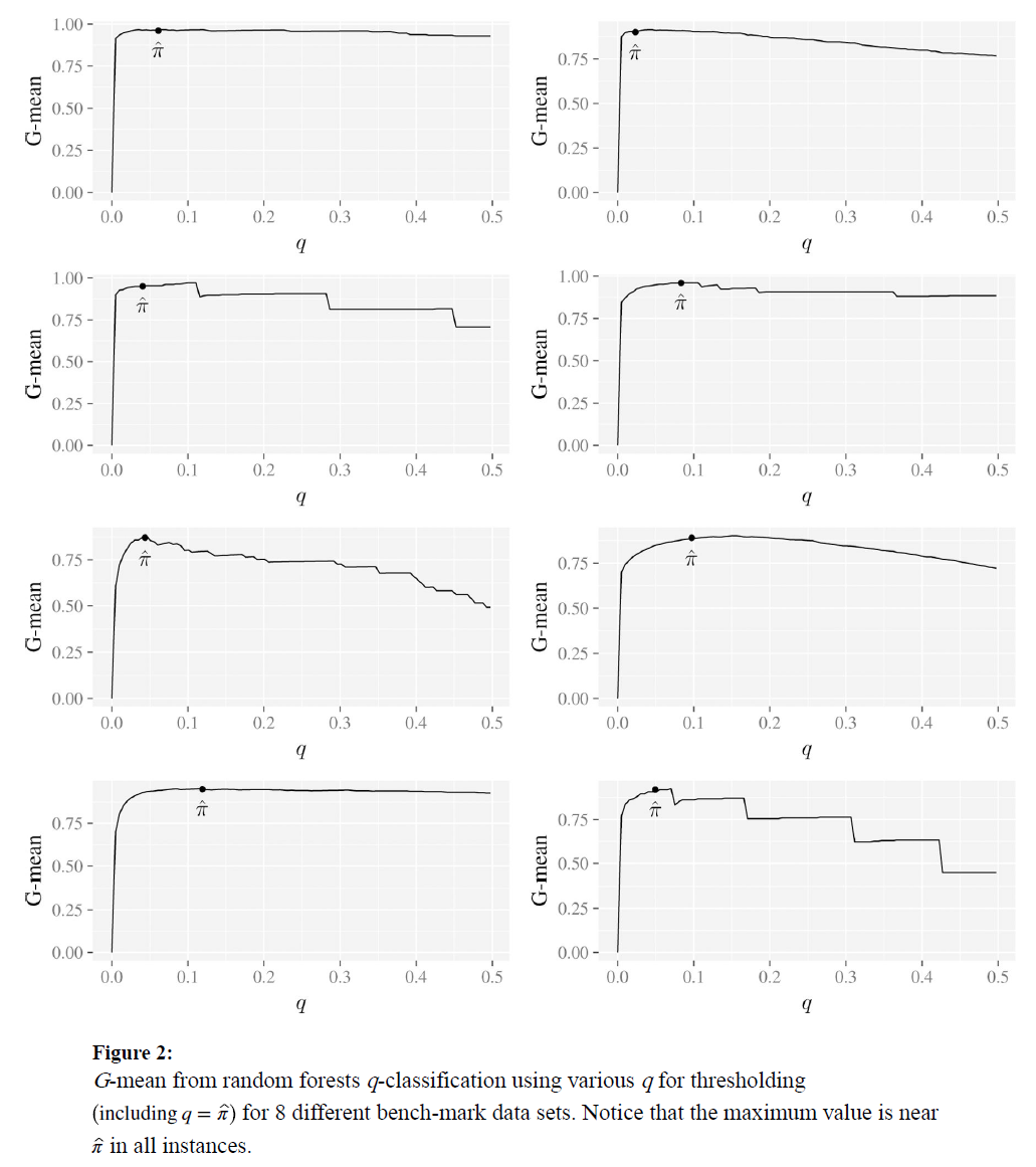
6-1. G-mean

$$\mbox{G-mean} = (TNR \times TPR)^{1/2}$$

q가 근사적으로 $\hat{\pi}$에 가까워졌을 때, RFQ에 의한 G-mean이 최대치에 가깝다는 것을 143개의 벤치마크 데이터셋을 통해서 확인했다.(10-fold CV를 250번씩 시행하였다.) 이는 분류기에 있어서 TNR+TPR optimality가 중요한 특징이라는 것을 시사한다.

(splitting criterion으로서 Gini index 대신 Hellinger distance를 사용해보긴 하였으나 크게 유의미하지는 않았다.)

6-2. ex1) Simulated data

epoch: 250, trees: 5000, nodesize=1, mtry=d/3

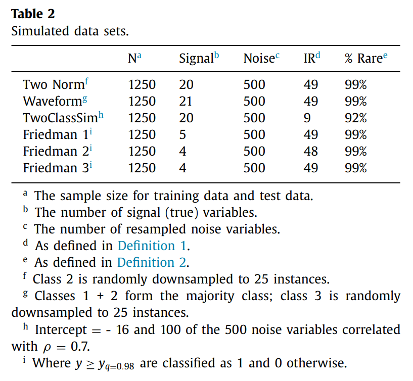
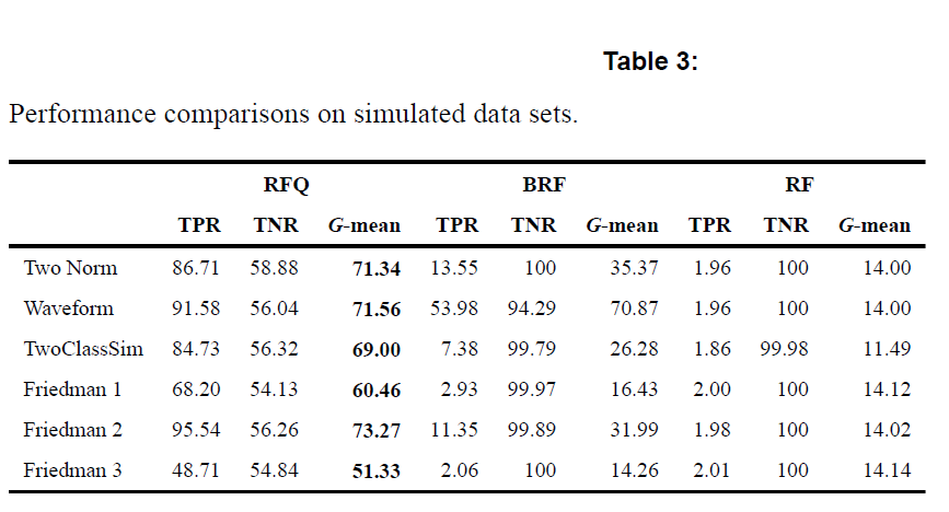
위 Table은 complex imbalanced data in high dimensional settings에서 RFQ가 효과적임을 보여주고 있다.

6-3. ex2) Cognitive impairment data

Alzheimers Disease CSF Data from AppliedPredictiveModeling (N=333, d=130 where $N_0=242, N_1=91$ with IR=2.66)

epoch: 250, trees: 5000, nodesize=1, mtry=d/3

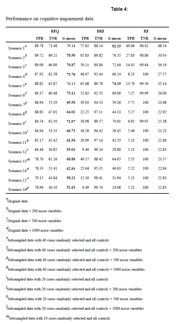
BRF의 경우에는 high dimensional이 될수록 성능이 낮아짐을 알 수 있다.

6-4. ex3) Customer churn data

N=3333 with $N_1=483$ and IR=5.90
epoch: 250, trees: 5000, nodesize=1, mtry=d/3

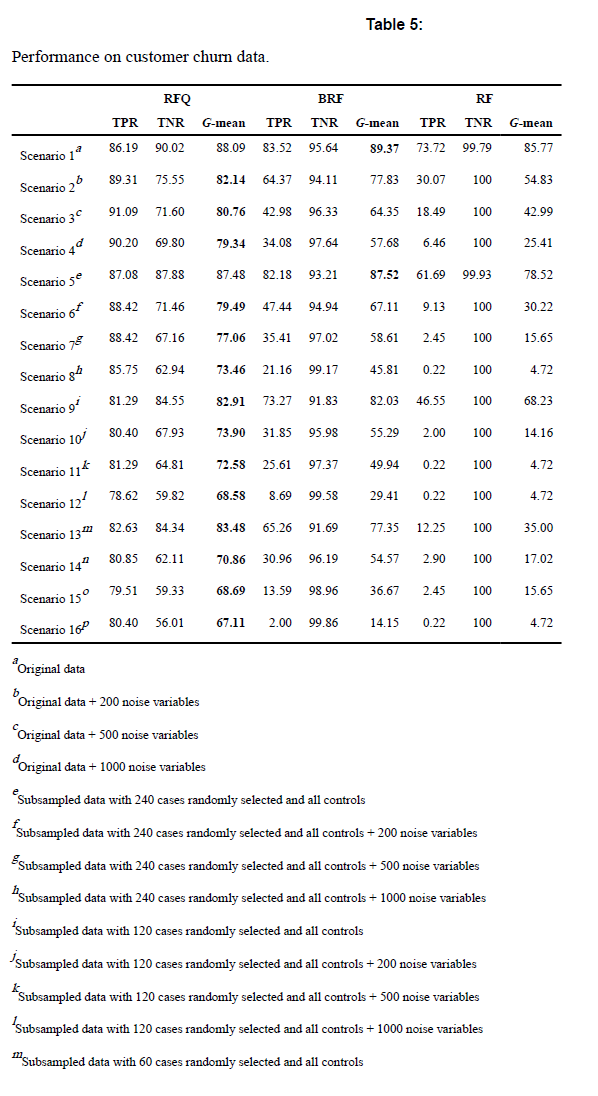
6-3와 같이, BRF는 high dimension일 때 성능이 좋지 않아짐을 알 수 있다.

6-5. Multiclass Imbalanced Data

Binary가 아니라 Multiclass의 경우에도 RFQ가 잘 작동하는지 확인해보았다.

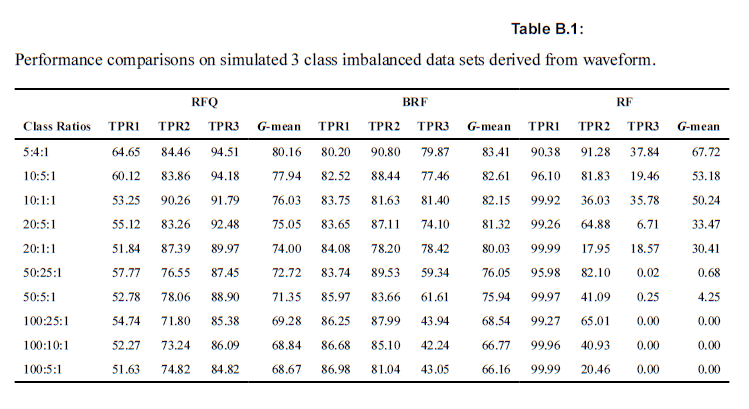
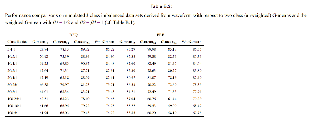
6-5-1. ex1) Waveform simulations

$$\mbox{weighted G-mean} = \Big(TPR1^{\beta_1} + TPR2^{\beta_2} + TPR3^{\beta_3}\Big)^{1/(\beta_1+\beta_2+\beta_3)}$$

2개 아니라, 3개의 클래스로 나누어져있는 경우에 G-mean을 통해 세 모델을 분류하였다. \(\binom{3}{2} = 3\)이므로, 총 세 경우의 수에 있어서 TPR과 TNR을 계산한 후 weighted G-mean을 계산하였다. 아래의 두 테이블의 차이는 각 그룹별 TPR의 가중치를 어떻게 두고 G-mean을 계산했는지에 따라 다르다. 참고로 unweighted G-mean은 multiclass 상황에서 적절하지는 않다. 특히 심각한 불균형이 존재할 경우 더욱 그러하다. 아래의 경우에는 \(\beta_1, \beta_2, \beta_3\)를 각각 러프하게 1/2, 1, 1로 넣었지만, 이는 저자가 의도하는 바를 담기에는 충분한 차이를 보이긴 했다. 아래의 표를 통해서 구체적인 수치를 확인해보도록 하자.

6-5-2. ex2) Cassini simulations

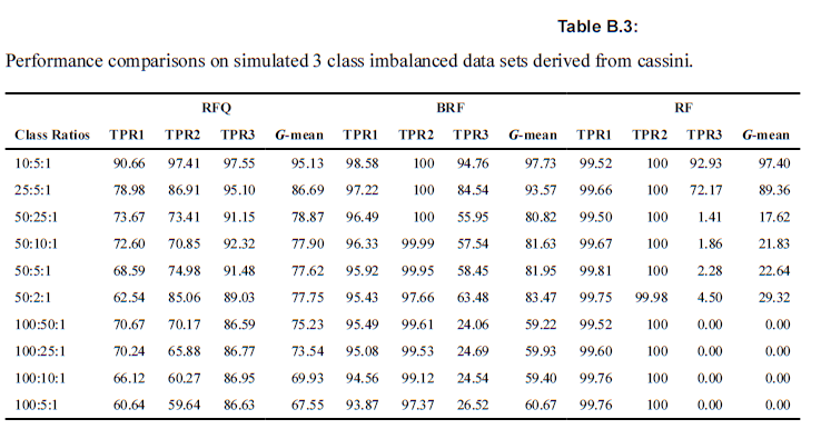
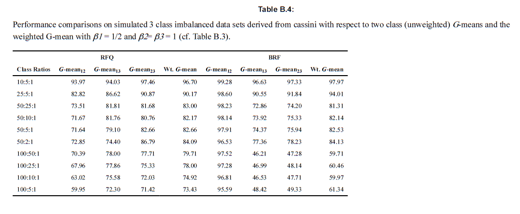
위의 예시와 시사하는 바는 동일하다.

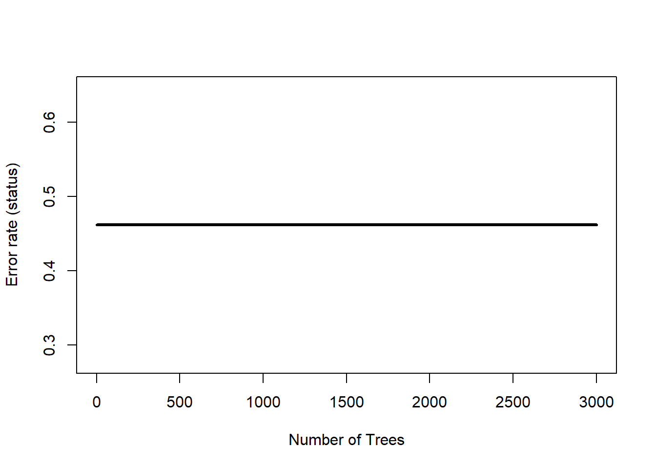
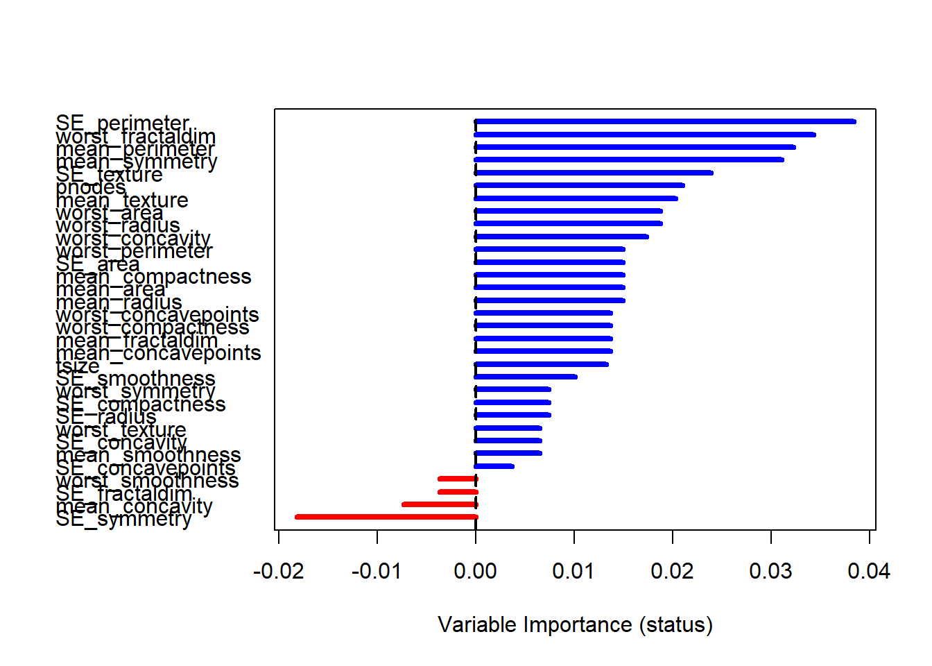
7. Variable Importance

• Breiman-Culter importance(tree-based) : not fit
  대부분의 노트들이 0을 갖고 있을 것이기 때문에 불균형데이터에서는 해당 기준으로 VIMP을 나타내는 데에는 적절하지 못하다.

• G-mean with Ishwaran-Kogalur importance(ensemble) : do fit
  blocked ensemble의 prediction error를 통해서 계산한다.

1

library(randomForestSRC)

## Warning: 패키지 'randomForestSRC'는 R 버전 3.6.3에서 작성되었습니다

## 
##  randomForestSRC 2.11.0 
##  
##  Type rfsrc.news() to see new features, changes, and bug fixes. 
## 

1
2
3
4

data(breast)
breast <- na.omit(breast)
o.rfq <- imbalanced(status ~ ., breast, importance = TRUE)
print(o.rfq)

##                          Sample size: 194
##            Frequency of class labels: 148, 46
##                      Number of trees: 3000
##            Forest terminal node size: 1
##        Average no. of terminal nodes: 27.20167
## No. of variables tried at each split: 6
##               Total no. of variables: 32
##        Resampling used to grow trees: swor
##     Resample size used to grow trees: 123
##                             Analysis: RFQ
##                               Family: class
##                       Splitting rule: gini *random*
##        Number of random split points: 10
##               Normalized brier score: 73.24 
##                                  AUC: 55.29 
##                               G-mean: 0.54
##                     Imbalanced ratio: 3.22
##                           Error rate: 0.46
## 
## Confusion matrix:
## 
##           predicted
##   observed  N  R class.error
##          N 73 75      0.5068
##          R 19 27      0.4130
## 
## 	Overall error rate: 46.19%

1

plot(o.rfq, plots.one.page = FALSE)

## 
##                       Importance   Relative Imp
## SE_perimeter              0.0384         1.0000
## worst_fractaldim          0.0343         0.8932
## mean_perimeter            0.0322         0.8401
## mean_symmetry             0.0311         0.8098
## SE_texture                0.0239         0.6223
## pnodes                    0.0210         0.5480
## mean_texture              0.0203         0.5295
## worst_area                0.0188         0.4889
## worst_radius              0.0188         0.4889
## worst_concavity           0.0173         0.4521
## worst_perimeter           0.0149         0.3897
## SE_area                   0.0149         0.3897
## mean_compactness          0.0149         0.3897
## mean_area                 0.0149         0.3897
## mean_radius               0.0149         0.3897
## worst_concavepoints       0.0137         0.3568
## worst_compactness         0.0137         0.3568
## mean_fractaldim           0.0137         0.3568
## mean_concavepoints        0.0137         0.3568
## tsize                     0.0133         0.3459
## SE_smoothness             0.0101         0.2622
## worst_symmetry            0.0074         0.1935
## SE_compactness            0.0074         0.1935
## SE_radius                 0.0074         0.1935
## worst_texture             0.0065         0.1683
## SE_concavity              0.0065         0.1683
## mean_smoothness           0.0065         0.1683
## SE_concavepoints          0.0037         0.0964
## worst_smoothness         -0.0037        -0.0958
## SE_fractaldim            -0.0037        -0.0958
## mean_concavity           -0.0073        -0.1909
## SE_symmetry              -0.0181        -0.4724

1

# get.imbalanced.performance(o.rfq) # 언제부터인가 없어졌다.

8. Comparison to Boosting

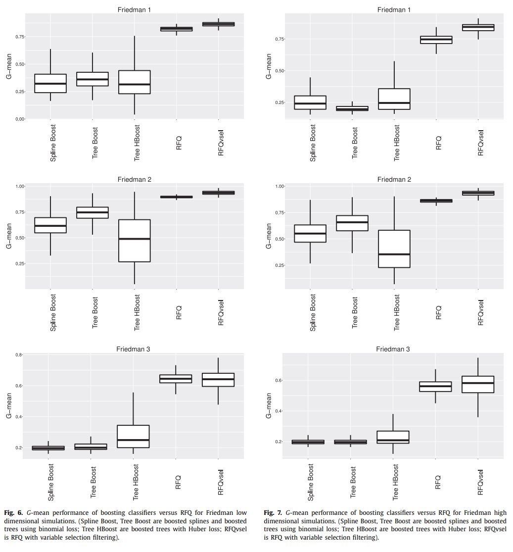
Figure 6 and 7 are the cases of low or high dimensional task, respectively.

• Spline Boost: boosted parametric splines using binomial loss
• Tree Boost: boosted trees using binomial loss (nonparametric boosting)
• Tree HBoost: boosted trees using Huber loss (nonparametric boosting)
• RFQ: Random Forest with q-classifier
• RFQvsel: RFQ with variable selection

9. Discussion

high complexity, high imbalancedness, high dimensionality에서 RFQ가 효과적이었다.
BRF가 아직 계산이 더 빠르기는 하지만 큰 차이는 아니다. 심지어 Theorem 4에 의해 subsampling을 한다면 computational load도 줄이면서 TNR+TPR optimal은 놓치지 않을 수 있다.

10. Further Reference

불균형데이터에 대해서 알고 싶다면 아래의 세 논문을 추가 참고해보면 좋을 것 같다.

1. Krawczyk, B. (2016). Learning from imbalanced data: open challenges and future directions. Progress in Artificial Intelligence, 5(4), 221-232.
2. Haixiang, G., Yijing, L., Shang, J., Mingyun, G., Yuanyue, H., & Bing, G. (2017). Learning from class-imbalanced data: Review of methods and applications. Expert Systems with Applications, 73, 220-239.
3. Das, S., Datta, S., & Chaudhuri, B. B. (2018). Handling data irregularities in classification: Foundations, trends, and future challenges. Pattern Recognition, 81, 674-693.

이 논문에 대해서 영어로 정리된 깃헙 페이지가 있다.

—

Critical Point (MY OWN OPINION)

1. 중간에도 언급했지만, Bayesian의 용어로 해석한다면, uniform prior가 아니라 likelihood를 기준으로 분류를 했다는 데에 의의가 있는 것 같다. 달리 말하면, 단순히 classifier의 threshold를 1/2이 아닌 \(\pi\)로 했다고 볼 수 있지만, 그 이면의 수학적 의미를 잘 증명해낸 논문이라고 생각한다.

2. G-mean을 performance metrics로써 활용할 때, 가중평균을 사용하면 조금 더 좋은 결과를 얻게 되지 않을까? 예를 들어, TPR에 조금 더 가중치를 두어서 \(\mbox{weighted G-mean} = TNR^{0.2} \times TPR^{0.8}\)처럼?

3. Regression 문제에는 이 아이디어를 어떻게 활용할 수 있을까?

—