Torgo, L., & Ribeiro, R. (2007, September). Utility-based regression. In European conference on principles of data mining and knowledge discovery (pp. 597-604). Springer, Berlin, Heidelberg.

In Short

It is about the metrics which is useful when there is the prediction of rare extreme values of a continuous target variable. Kind of cost-sensitive learning.

1. Introduction

Regression 상황에서 benefit과 cost를 정의하고 이 둘의 차를 utility라고 정의한다.

2. Problem Formulation

1. Regression에서 Uniform cost assumption은 비현실적이다. 현실에서는 cost-sensitive learning이 필요한 경우가 더 많다.
2. 그리고 Classification에서는 class에 따라서 cost를 다르게 적용하는 데에 반해, Regression에서는 그러하지 않다. (뭉쳐있는 데이터에서 error가 크게 발생한 것과, 따로 떨어져있는 데이터에서 error가 크게 발생한 것을 구분해야 한다는 이야기이다.)
3. 기존의 regression에서 non-uniform cost assumption를 연구한 것은 대체로 under-prediction과 over-prediction을 구분하는 데에 그쳤다.
4. cost뿐만 아니라, benefit에 대해서도 고려해야 한다.
5. 결론: Relevance(Importance)를 정의하여 cost를 새롭게 정의할 필요성이 있다.

3. Utility-Based Regression

3-1. Relevance Functions

$$\phi(Y): \mathscr{R} \rightarrow0..1$$

Utility-based regression is independent of the shape of the \(\phi()\) function. 기존적으로는 user가 relevance를 정의하는 것이 가장 좋지만, 그렇지 못한 데이터가 현실에서는 대부분이다. Relevance는 대부분의 경우 Rarity(희소성)과 관련이 있다. 기본적으로는 target variable의 pdf에 반비례하게끔 설정하면 되지만, 그 pdf를 추정하는 것이 어렵다.

3-2. Cost and Benefit Surfaces

3-2-1. Utility of Prediction

$$U = TB - TC \\ \text{where TB and TC are total benefit and total cost, respectively}$$

3-2-2. Cost of Prediction

$$TC = \sum^{n}_{i=1}c(\hat{y_i},y) \\ \text{where } c(\hat{Y},Y) = \Phi(\hat{Y},Y) \times C_{\max} \times L(\hat{Y},Y)$$

Cost of prediction depends on three components. One is the relevance of the test case value, and the others are the relevance of the predicted value and precision of the prediction. 여기서 relevance of the test case value는 \(\phi(Y)\)이고, relevance of the predicted value는 \(\phi(\hat{Y})\)이다. 이와 관련하여 아래 유의사항 세 가지가 있다.

1. False Alarm: Predict a relevant value for an irrelevant test case
2. Oppotunity Cost: Predict an irrelevant value for a relevant test case
3. Confusing Relevant Events(the most serious mistakes): Predict a relevant but very different value for a relevant test case

(i) Bivariate Relevance Function \(\Phi(\hat{Y},Y)\)
1과 2를 고려하기 위해서 Bivariate Relevance Function를 아래와 같이 정의한다. m은 0과 1사이의 값을 갖는 hyperparameter인데, False Alarm(1)보다 Oppotunity Cost(2)를 더욱 중요하게 보고 싶은 경우 0.5 이상의 값을 설정하면 된다.

$$\Phi(\hat{Y},Y) = (1-m) \cdot \phi(\hat{Y}) + m \cdot \phi(Y)$$

(ii) Maximum Cost \(C_{\max}\)
maximum cost that is only assigned when the relevance of the prediction is maximum (i.e. \(\Phi(\hat{Y},Y)=1\)). Usually, \(C_{\max}\) is provided as a constant by the user.

(iii) Loss Function \(L(\hat{Y},Y)\)
아무 metric이나 써도 되긴 하지만, 해석을 용이하게 하기 위해서 0부터 1사이 값을 권장한다. \(\Phi(\hat{Y},Y) \times C_{\max}\)은 발생가능한 최악의 상황에서의 최대 페널티 값을 의미하기 때문이다. (the maximum penalty we get if \(\hat{Y}\) is the worst possible prediction.) 즉, \(L(\hat{Y},Y)=1\)이면 최대 cost가 되는 것이다. 반면, \(L(\hat{Y},Y)=0\)이면, relevance와 상관없이 cost는 0이다. 아래는 논문 저자가 제안하는 Loss function이다.

$$L(\hat{Y},Y) = \Big| \max_{i \in \hat{Y}..Y} \phi(i) - \min_{i \in \hat{Y}..Y} \phi(i)\Big|$$

3-2-3. Benefit of Prediction

$$TB = \sum^{n}_{i=1}b(\hat{y_i},y) \\ \text{where } b(\hat{Y},Y) = \phi(Y) \times B_{\max} \times \Big(1-L(\hat{Y},Y)\Big)$$

This definition of benefits associates higher rewards with higher relevance. \(\phi(Y) \times B_{\max}\)을 maximum benefit with relevance라고 생각하고, \(\Big(1-L(\hat{Y},Y)\Big)\)를 일종의 proportion이라고 생각하면 된다.

(i) Maximum Benefit \(B_{\max}\)
Like \(C_{\max}\), \(B_{\max}\) is a user-defined maximum reward which means it is a constant.

4. An Illustrative Application

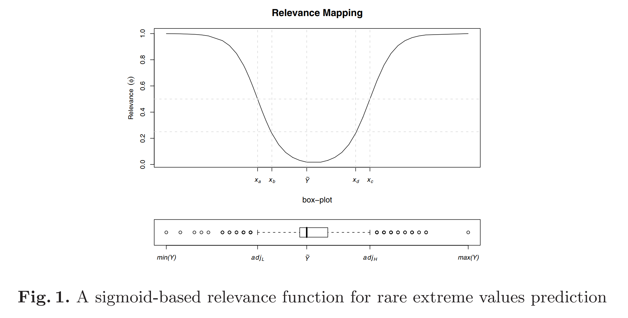
Boxplot의 정보를 활용하기
Simpler strategy to derive a relevance function for a class of application where relevance is associated with rarity: the prediction of rare extreme values of a numeric variable

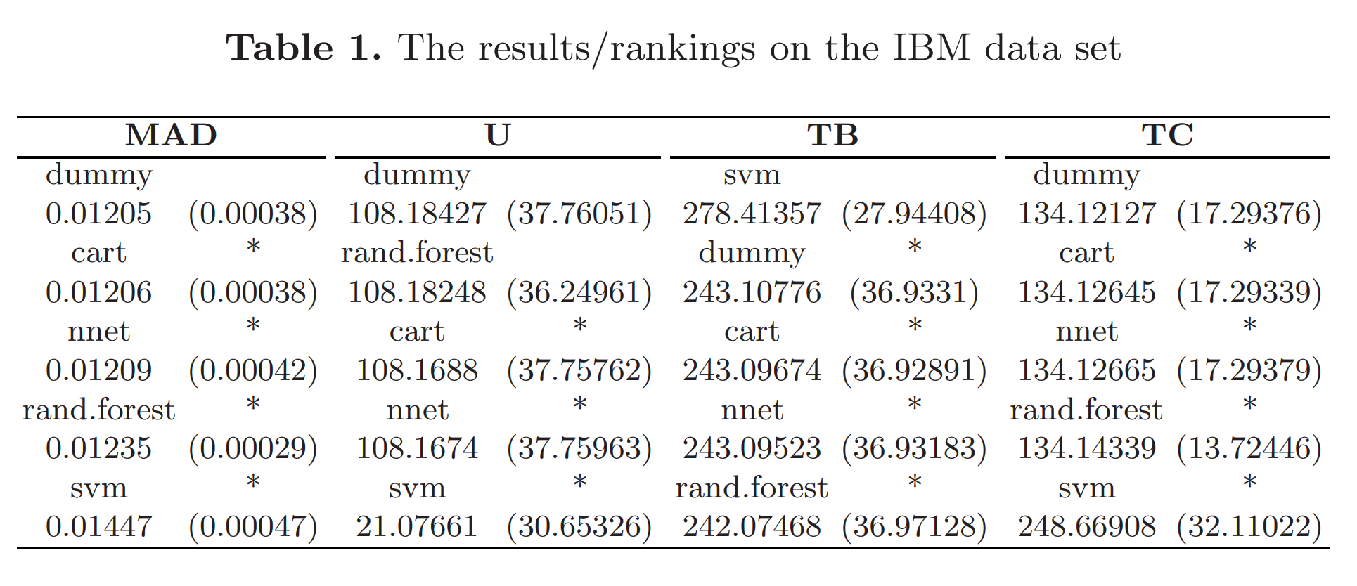
Table1을 보면, SVM이 TB는 높지만 TC도 높아서 U는 낮은 것을 볼 수 있다. 하지만, 본 연구의 핵심은 U를 높이는 것이 아니라, rare extreme value를 잘 예측했는지이다.

5. Conclusion

New evaluation frame work for regression tasks with non-uniform costs and benefits of the predictions.

—

Critical Point (MY OWN OPINION)

1. boxplot을 활용하면, 놓지는 부분이 많을 것 같다. 특히, gaussian mixture model을 따를 경우, 중앙값이 이들을 충분히 대변하지 못할 수 있다. KDE를 하면 더 좋지 않을까?

2. 그리고, 추후 SMOTE for Regression에서 활용할 때, relevance function을 통해서 0과 1로 classification 문제로 변형할 때 생길 수 있는 문제점은 어떠한 것이 있을까?

3. hyperparameter로는 \(C_{\max}, B_{\max}, m\)와 같은 것들이 있는데, 특히 \(C_{\max}\)와 \(B_{\max}\)에 대한 사전지식이 없을 경우 이 둘을 어떠한 비율로 설정하는지도 중요할 것 같다.

—

ETC

• R에서는 uba라는 패키지로 구현되어 있다. 자세한 사항은 해당 사이트를 참고해보면 된다.
• 추후 https://www.dcc.fc.up.pt/~rpribeiro/publ/rpribeiroPhD11.pdf를 꼭 읽어볼 것.