y <- c(93, 112, 122, 135, 122, 150, 118, 90, 124, 114)
n <- length(y)
s2 <- var(y)
my <- mean(y)
# helper functions to sample from and evaluate
# scaled inverse chi-squared distribution
rsinvchisq <- function(n, nu, s2, ...) nu*s2 / rchisq(n , nu, ...)
dsinvchisq <- function(x, nu, s2){
  exp(log(nu/2)*nu/2 - lgamma(nu/2) + log(s2)/2*nu - log(x)*(nu/2+1) - (nu*s2/2)/x)
}

ns <- 1000
sigma2  <- rsinvchisq(ns, n-1, s2)
mu <- my + sqrt(sigma2/n)*rnorm(length(sigma2))
sigma <- sqrt(sigma2)
ynew <- rnorm(ns, mu, sigma)

t1l <- c(90, 150)
t2l <- c(10, 60)
nl <- c(50, 185)
t1 <- seq(t1l[1], t1l[2], length.out = ns)
t2 <- seq(t2l[1], t2l[2], length.out = ns)
xynew <- seq(nl[1], nl[2], length.out = ns)

# multiplication by 1./sqrt(s2/n) is due to the transformation of
# variable z=(x-mean(y))/sqrt(s2/n), see BDA3 p. 21
pm <- dt((t1-my) / sqrt(s2/n), n-1) / sqrt(s2/n)
pmk <- density(mu, adjust = 2, n = ns, from = t1l[1], to = t1l[2])$y

# the multiplication by 2*t2 is due to the transformation of
# variable z=t2^2, see BDA3 p. 21
ps <- dsinvchisq(t2^2, n-1, s2) * 2*t2
psk <- density(sigma, n = ns, from = t2l[1], to = t2l[2])$y

# multiplication by 1./sqrt(s2/n) is due to the transformation of variable
# see BDA3 p. 21
p_new <- dt((xynew-my) / sqrt(s2*(1+1/n)), n-1) / sqrt(s2*(1+1/n))

# Combine grid points into another data frame
# with all pairwise combinations
dfj <- data.frame(t1 = rep(t1, each = length(t2)),
                  t2 = rep(t2, length(t1)))
dfj$z <- dsinvchisq(dfj$t2^2, n-1, s2) * 2*dfj$t2 * dnorm(dfj$t1, my, dfj$t2/sqrt(n))
# breaks for plotting the contours
cl <- seq(1e-5, max(dfj$z), length.out = 6)
Demo 3.1
dfm <- data.frame(t1, Exact = pm, Empirical = pmk) %>% gather(grp, p, -t1)
margmu <- ggplot(dfm) +
geom_line(aes(t1, p, color = grp)) +
coord_cartesian(xlim = t1l) +
labs(title = 'Marginal of mu', x = '', y = '') +
scale_y_continuous(breaks = NULL) +
theme(legend.background = element_blank(),
legend.position = c(0.75, 0.8),
legend.title = element_blank())
dfs <- data.frame(t2, Exact = ps, Empirical = psk) %>% gather(grp, p, -t2)
margsig <- ggplot(dfs) +
geom_line(aes(t2, p, color = grp)) +
coord_cartesian(xlim = t2l) +
coord_flip() +
labs(title = 'Marginal of sigma', x = '', y = '') +
scale_y_continuous(breaks = NULL) +
theme(legend.background = element_blank(),
legend.position = c(0.75, 0.8),
legend.title = element_blank())
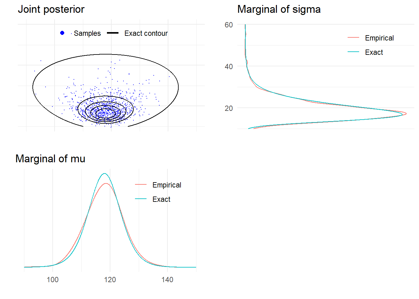
joint1labs <- c('Samples','Exact contour')
joint1 <- ggplot() +
geom_point(data = data.frame(mu,sigma), aes(mu, sigma, col = '1'), size = 0.1) +
geom_contour(data = dfj, aes(t1, t2, z = z, col = '2'), breaks = cl) +
coord_cartesian(xlim = t1l,ylim = t2l) +
labs(title = 'Joint posterior', x = '', y = '') +
scale_y_continuous(labels = NULL) +
scale_x_continuous(labels = NULL) +
scale_color_manual(values=c('blue', 'black'), labels = joint1labs) +
guides(color = guide_legend(nrow = 1, override.aes = list(
shape = c(16, NA), linetype = c(0, 1), size = c(2, 1)))) +
theme(legend.background = element_blank(),
legend.position = c(0.5, 0.9),
legend.title = element_blank())
grid.arrange(joint1, margsig, margmu, nrow = 2)