Monte Carlo Method

Chapter 04.
Monte Carlo Approximation

본 포스팅은 First Course in Bayesian Statistical Methods를 참고하였다.

Monte Carlo Method

Monte Carlo Method는 이름은 거창해보이지만 사실 그 방법은 매우 간단하다.
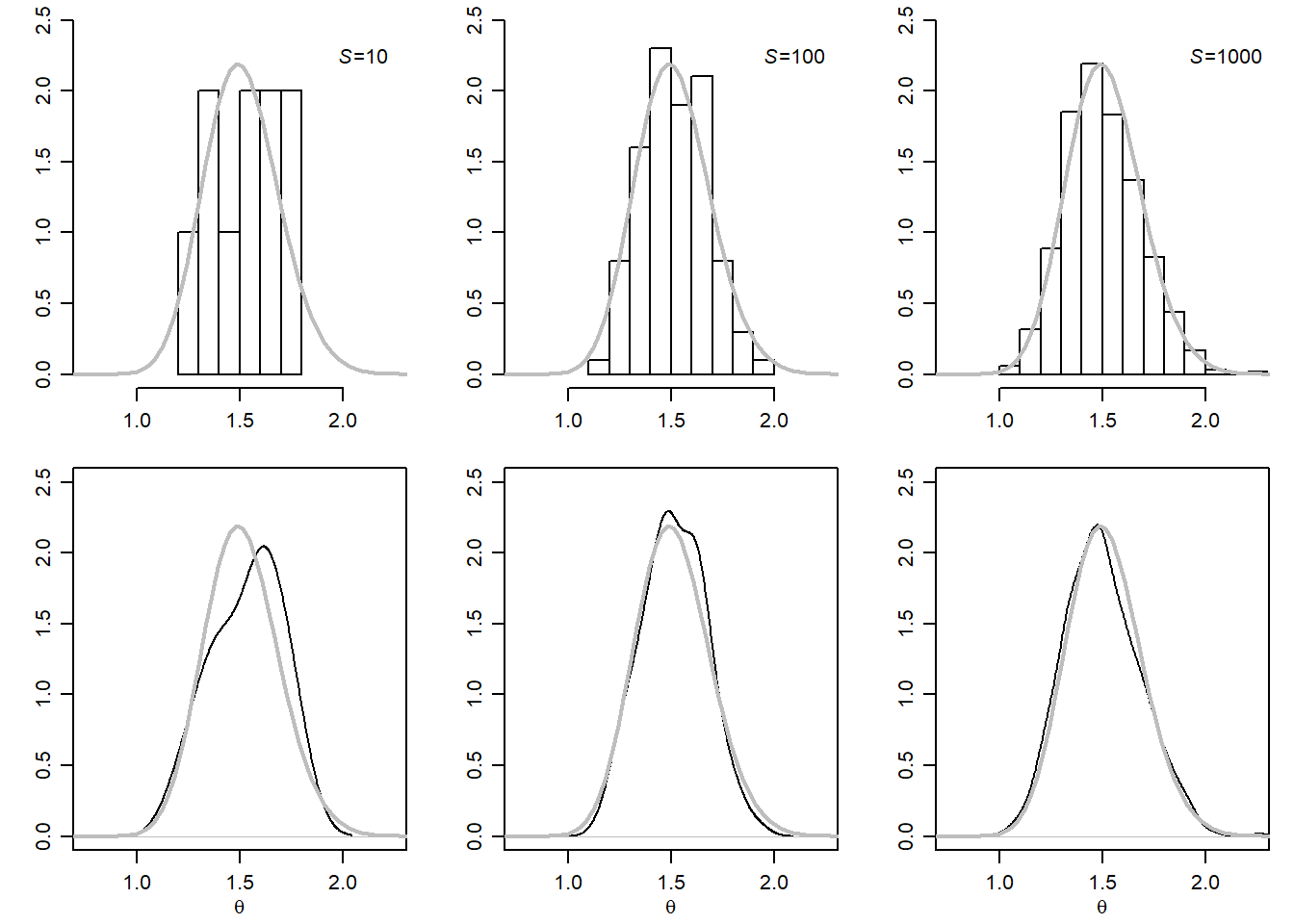
우선, 사후분포( $p(\theta|y_1,...,y_n)$ )로부터 S개의 random sample을 뽑는다.
$$\theta^{1}, …, \theta^{S} \ \stackrel{iid}{\sim} \ p(\theta|y_1, …, y_n) $$
그러면 S가 커질수록 { $\theta^{1}, ..., \theta^{S}$ }는 근사적으로 사후분포( $p(\theta|y_1,...,y_n)$ )를 따른다.
이를 통해 $E[\theta|y_1, ..., y_n]$ , $Var[\theta|y_1, ..., y_n]$ 부터 중앙값, $\alpha$ percentile 등의 통계량값들을 근사적으로 계산할 수 있다.

이때 approximate Monte Carlo Standard error은 $\sqrt{\hat{\sigma}^2/S}$ 이다. 그렇기 때문에, 가령 $E[\theta|y_1, ..., y_n]$ 와 Monte Carlo 추정치의 차이가 0.01이하로 하고 싶다고 한다면, Monte Carlo Sample Size를 조정해주면 된다. 이때 예를 들어서 $\hat{\sigma}^2$ 가 0.024라고 한다면, Sample Size는 $2\sqrt{0.024/S} < 0.01$ 로 계산해서 sample을 960개보다는 많이 뽑아야 함을 알 수 있다.

Monte Carlo Method를 활용하면 다양한 것들을 할 수 있는데, 그 대표적인 예시로 아래 세 개를 이해해보자.

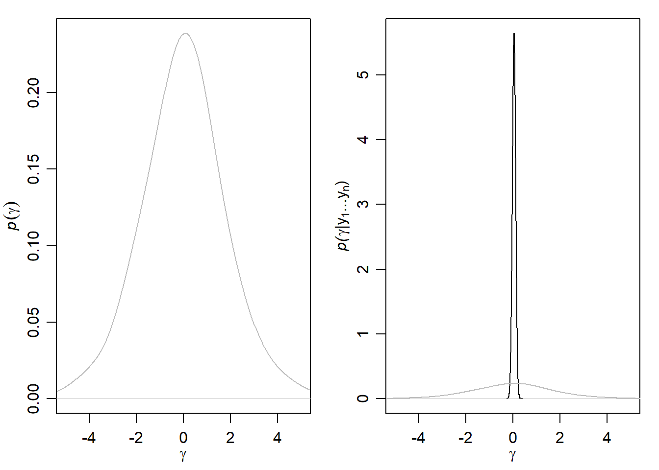
1. Posterior Inference for Arbitrary Functions

$\theta$ 그 자체가 아니라 임의의 $f(\theta)$ 의 posterior distribution이 궁금할 수 있다. 예를 들어서, log odds와 같은 것 말이다. 하지만 결국 $\gamma = f(\theta)$ 도 $\theta$ 처럼 Monte Carlo Method로 사후분포을 추정할 수 있다.

하나의 parameter만 있는 것이 아니라, 심지어 $Pr(\theta_1 > \theta_2 | Y_{1,1} = y_{1,1}, ..., Y_{n_2,2}=y_{n_2,2})$ 나 $Pr(\theta_1/\theta_2 | Y_{1,1} = y_{1,1}, ..., Y_{n_2,2}=y_{n_2,2})$ 처럼 parameter가 두 개인 경우도 구할 수 있다.

2. Sampling from Predictive Distributions

Step1. sample $\theta^{(1)},...,\theta^{(S)} \text{ ~ i.i.d} \ p(\theta|y_1,...,y_n)$
Step2. approximate $p(\tilde{y}|y_1,...,.y_n)$ with $\sum_{s=1}^{S}p(\tilde{y}|\theta^{(s)})/S$

위 방법을 통해 $Pr(\tilde{Y_1}>\tilde{Y_2}|\sum Y_{i,1}=217,\sum Y_{i,2}=66)$ 를 근사하는 것도 가능하다. 왜냐하면 $Pr(\tilde{Y_1})$ 와 $Pr(\tilde{Y_2})$ 은 posterior independent하기 때문이다.

 1
 2
 3
 4
 5
 6
 7
 8
 9
10
11
12


set.seed(1)
a<-2 ; b<-1
sy1<-217 ;  n1<-111
sy2<-66  ;  n2<-44

theta1.mc<-rgamma(10000,a+sy1, b+n1)
theta2.mc<-rgamma(10000,a+sy2, b+n2)

y1.mc<-rpois(10000,theta1.mc)
y2.mc<-rpois(10000,theta2.mc)

mean(theta1.mc>theta2.mc)

## [1] 0.9708

1

mean(y1.mc>y2.mc)

## [1] 0.4846

위 결과를 통해서 주의깊게 살펴보아야 할 것은, 예측치의 차이와 모수의 차이가 같지 않다는 점이다.

아래 세 개 구분하기

(1) sampling model: $Pr(\tilde{Y}=\tilde{y}|\theta)$
(2) prior predictive model: $Pr(\tilde{Y}=\tilde{y})$
- $\theta$ 에 대한 사전확률분포가 관측가능한 데이터 $\tilde{Y}$ 에 대해 합리적인 믿음을 나타낼 수 있는지 확인해보는 용도로 활용가능하다.
(3) posterior predictive model: $Pr(\tilde{Y}=\tilde{y}|Y_1=y_1, ..., Y_n=y_n)$

3. Posterior Predictive Model Checking

We should at least make sure that our model generates predictive datasets $\tilde{Y}$ that resemble the observed dataset in terms of features that are of interest

1
2
3


load("gss.RData")

table(gss$DEG[gss$YEAR==1998])

## 
##    0    1    2    3    4 
##  430 1500  209  478  205

1
2
3
4
5
6


y1<-gss$PRAYER[gss$YEAR==1998 & gss$RELIG==1 ]
y1<-1*(y1==1)
y1<-y1[!is.na(y1) ]
sy1<-sum(y1)
n1<-length(y1)
sy1/n1

## [1] 0.3616803

1
2
3
4
5
6


y2<-gss$PRAYER[gss$YEAR==1998 & gss$RELIG!=1 ]
y2<-1*(y2==1)
y2<-y2[!is.na(y2) ]
sy2<-sum(y2)
n2<-length(y2)
sy2/n2

## [1] 0.5471464

1

table(gss$FEMALE[gss$YEAR==1998])

## 
##    0    1 
## 1232 1600

1
2
3
4
5
6


y<-gss$FEMALE[gss$YEAR==1998]
y<-1*(y==1)
y<-y[!is.na(y) ]
sy<-sum(y)
n<-length(y)
sy/n

## [1] 0.5649718

1
2
3


sy<-sy2
n<-n2
sy/n

## [1] 0.5471464

 1
 2
 3
 4
 5
 6
 7
 8
 9
10
11
12
13
14
15
16
17
18
19
20
21
22
23


#### MC approximations
set.seed(1)

a<-1 ; b<-1 
theta.prior.sim<-rbeta(10000,a,b)
gamma.prior.sim<- log( theta.prior.sim/(1-theta.prior.sim) )

n0<-860-441 ; n1<-441
theta.post.sim<-rbeta(10000,a+n1,b+n0)
gamma.post.sim<- log( theta.post.sim/(1-theta.post.sim) )

par(mar=c(3,3,1,1),mgp=c(1.75,.75,0))
par(mfrow=c(2,3))
par(cex=.8)

par(mfrow=c(1,2),mar=c(3,3,1,1), mgp=c(1.75,.75,.0))
plot(density(gamma.prior.sim,adj=2),xlim=c(-5,5),main="", 
     xlab=expression(gamma),
     ylab=expression(italic(p(gamma))),col="gray")
plot(density(gamma.post.sim,adj=2),xlim=c(-5,5),main="",xlab=expression(gamma),
     ylab=expression(paste(italic("p("),gamma,"|",y[1],"...",y[n],")",
                           sep="")) )
lines(density(gamma.prior.sim,adj=2),col="gray")

 1
 2
 3
 4
 5
 6
 7
 8
 9
10
11
12
13
14
15
16
17
18
19
20
21
22
23
24
25
26
27


set.seed(1)
a<-2 ; b<-1
sy1<-217 ;  n1<-111
sy2<-66  ;  n2<-44

theta1.mc<-rgamma(10000,a+sy1, b+n1)
theta2.mc<-rgamma(10000,a+sy2, b+n2)

y1.mc<-rpois(10000,theta1.mc)
y2.mc<-rpois(10000,theta2.mc)

#### Posterior predictive check 
y1<-gss$CHILDS[gss$FEMALE==1 &  gss$YEAR>=1990  & gss$AGE==40 & gss$DEG<3 ]
y1<-y1[!is.na(y1)]

set.seed(1)

a<-2 ; b<-1
t.mc<-NULL
for(s in 1:10000) {
  theta1<-rgamma(1,a+sum(y1), b+length(y1))
  y1.mc<-rpois(length(y1),theta1)
  t.mc<-c(t.mc,sum(y1.mc==2)/sum(y1.mc==1))
}

t.obs<-sum(y1==2)/sum(y1==1)
mean(t.mc>=t.obs)

## [1] 0.0049

 1
 2
 3
 4
 5
 6
 7
 8
 9
10
11
12
13
14
15
16
17
18
19
20


par(mar=c(3,3,1,1),mgp=c(1.75,.75,0))
par(mfrow=c(1,2))

ecdf<-(table(c(y1,0:9))-1 )/sum(table(y1))
#ecdf.mc<-(table(c(y1.mc,0:9))-1 )/sum(table(y1.mc))
ecdf.mc<- dnbinom(0:9,size=a+sum(y1),mu=(a+sum(y1))/(b+length(y1)))
plot(0:9+.1,ecdf.mc,type="h",lwd=5,xlab="number of children",
     ylab=expression(paste("Pr(",italic(Y[i]==y[i]),")",sep="")),col="gray",
     ylim=c(0,.35))
points(0:9-.1, ecdf,lwd=5,col="black",type="h")

legend(1.8,.35,
       legend=c("empirical distribution","predictive distribution"),
       lwd=c(2,2),col=
         c("black","gray"),bty="n",cex=.8)


hist(t.mc,prob=T,main="",ylab="",xlab=expression(t(tilde(Y))) )

segments(t.obs,0,t.obs,.25,col="black",lwd=3)

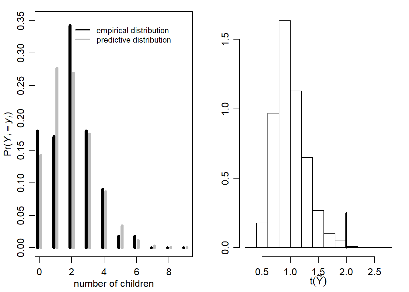
실제(empirical) 분포와 예측 분포의 모습이 다소 차이가 남을 확인할 수 있다.

참고

[1] FCB code

혹시 궁금한 점이나 잘못된 내용이 있다면, 댓글로 알려주시면 적극 반영하도록 하겠습니다.

Monte Carlo Method